Energy Savings and Payback Periods
As with other energy saving devices, the actual energy savings and payback periods for daylight harvesting with the IntelliBlinds™ Model D will depend on numerous installation-specific variables. The most significant of these are the type of daylight-harvesting lighting control, the amount of base-case window shading and lighting Energy Use Intensity (EUI), the width and height of the window, and the prevailing utility rates. Statistics on these variables can be readily used to project the distribution of savings and paybacks across any selected segment of the market. Such an analysis shows that IntelliBlinds™ will more than double the energy savings from daylight harvesting, while significantly shortening the payback periods and reducing payback uncertainties in typcal installations.
Energy Savings
The IntelliBlinds™ Model D saves energy in two ways:
- It automatically adjusts the shading in occupied spaces to maximize the average level of useful, glare-free daylight, boosting the savings from daylight harvesting.
- Because glare-free daylight is "cooler" than artificial light, the increased proportion of daylight reduces cooling loads on the building's HVAC system while the lights are "on". And because IntelliBlinds™ also adjusts the shading to minimize solar loads in unoccupied spaces, it reduces HVAC loads when the lights are "off", too.
In some buildings, the mean savings due to reduced HVAC loads can be 20–30% of the overall savings. However, HVAC savings are relatively difficult to estimate. For that reason—and for the sake of conservatism— the projections reported herein exclude any savings due to reduction of HVAC loads.
The IntelliBlinds™ Model D increases the energy saved through daylight harvesting because windows are generally over-shaded, drastically reducing the achievable savings. IntelliBlinds™ recovers the lost daylight by ensuring that the shading is always as open as possible without risk of glare or excessive brightness. The energy savings (kWh of electricity per square foot of daylit area per year) from daylight harvesting with IntelliBlinds™ can be projected as the product of two quantities:
- The relative savings from daylight harvesting with IntelliBlinds™
- The lighting Energy Use Intensity (EUI) in kiloWatt-hours per square foot per year (abbreviated herein as kWh/sf/yr) in sidelit areas
Relative Energy Savings
The relative (i.e. percentage) savings in lighting power and energy provided by IntelliBlinds™ depend mainly on three factors:
- The average level of daylight incident on the window.
- The degree to which the host window was shaded before installation of IntelliBlinds™.
- The type of daylight-harvesting lighting control IntelliBlinds™ is used with.
Average Level of Incident Daylight
With a window that receives little daylight (e.g. a north-facing window in the northern hemisphere), the daylight illuminance in the sidelit zone might only rarely approach the lighting control's set-point, even if the window is left completely unshaded. In such a scenario, the energy savings from daylight harvesting are limited by the average level of daylight incident on the window.
On the other hand, if the window receives enough daylight so that the unshaded illuminance often exceeds the lighting control's set-point, then the savings from daylight harvesting will typically be limited by the degree of window shading, rather than by the amount of incident daylight. This is the case with most windows in the continental USA that don't have a northern exposure. The savings, payback, and installed floor area projections for IntelliBlinds™ are based on this "shading-limited" scenario.
In the continental USA, the average year-round daytime horizontal daylight illuminance one window-head-height inward from an unshaded, non-north-facing window is about 500 lux, which also happens to be the typical lighting set-point illuminance in an office environment. And at just one-half window-head-heights away from the window, the average year-round daytime horizontal daylight illuminance rises to about 800 lux, or 1.6 typical lighting-control set-points.
So, if the daylight from sunny windows were always glare-free and had a constant illuminance, there would be virtually no need for artificial lighting in the sidelit areas. Unfortunately, the daytime daylight illuminance fluctuates over a wide range, forcing the use of window shading.
Degree of Base-Case Shading
The additional savings provided by IntelliBlinds™ depend on the degree of base-case shading, i.e. on how its host blind would have been used prior to IntelliBlinds™ installation. If the host blind would have always been fully raised, exposing the bare window glazing, then IntelliBlinds™ will provide no additional savings. On the other hand, if the host blind would have always been fully lowered with slats fully closed, then IntelliBlinds™ will dramatically boost the savings from daylight harvesting.
The degree of base-case shading will vary with occupant preferences (among other installation-specific factors). But windows with sunny exposures and manually operated Venetian blinds are generally heavily shaded in order to control glare.
One way to characterize the degree of shading provided by a Venetian blind is via the Relative Daylight Illuminance (RDI), which represents the ratio of the horizontal daylight illuminance at a desired point in the sidelit area to the illuminance that would result under the same conditions if the blinds were fully raised. The following curve plots the Cumulative Distribution Functions (CDFs) of RDIs with and without IntelliBlinds™ in sidelit areas in existing office buildings:
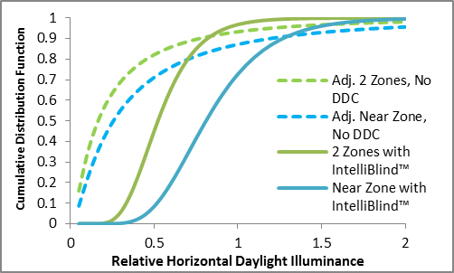
Two sets of curves are shown. The curves labeled "2 Zones" represent the CDFs of the RDI averaged over a sidelit area extending from 0.0 to 2.0 window-head-heights from the window. On the other hand, the curves labeled "Near Zone" represent the CDFs of the RDI averaged over a sidelit area extending from 0.0 to 1.0 window-head-heights from the window. The RDIs are normalized so that 1.0 represents the illuminance from an unshaded window averaged over the 2-zone area.
As the curves show, IntelliBlinds™ triples the median RDI—from 0.17 to 0.52 over two zones, and from 0.27 to 0.81 in the near zone.
The RDI represents a transfer function, i.e. the ratio of the actual horizontal daylight illuminance to the potential illuminance with an unshaded window. But, as previously discussed, the average year-round daytime horizontal daylight illuminance from an unshaded, non-north-facing window over a two-zone sidelit area is about 500 lux, or about 1.0 typical light-control set-points. Therefore, the RDI (i.e. x-axis) coordinates of Chart 1 can also be interpreted as the long-term average daylight illuminance, in lighting-control set-points, from sunny windows.
Type of Lighting Control
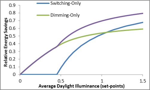
Of the many design variables that determine the ultimate energy saving performance of a daylight-harvesting lighting control, the most significant is whether it provides dimming-only, switching-only, or both dimming-and-switching control of the lighting load:
- Switching-Only (SO) controls save 100% of the lighting power when the daylight exceeds the set-point, but provide no savings when the daylight is less than the set-point.
- Dimming-Only (DO) controls can save energy when the daylight is less than the set-point, but can never save 100% of the lighting power because the lamps can be dimmed to no less than 5–10% of full brightness, and because ballast efficiency decreases as the lamps are dimmed.
- Dimming-and-Switching (D&S) controls are the best of both worlds: they include a dimming ballast to save energy when there's relatively little daylight, as well as a switch to reduce lighting power to zero when the daylight exceeds the set-point.
The following chart plots the relative energy savings versus average daylight illuminance (as a fraction of the lighting-control set-point) for each type of lighting control:
Cumulative Distribution Function (CDF) of Relative Savings
Because the RDI coordinates of Chart 1 can also be interpreted as average horizontal daylight illuminance values (in terms of lighting-control set-points), the RDI CDF curves can be used together with the relative energy savings curves of Chart 2 to determine the CDFs of relative energy savings.
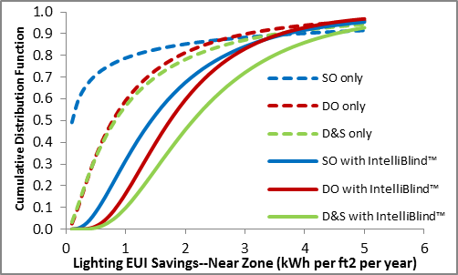
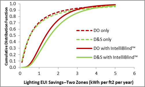
The following charts plot the CDFs of relative energy savings for different types of lighting control across potential sidelit areas in existing buildings in the continental USA. The first chart shows the CDFs for the near zone (ranging from 0.0 to 1.0 window-head-heights from the window), while the second chart shows the CDFs for the entire sidelit area comprising both near and far zones (ranging from 0.0 to 2.0 window-head-heights from the window):
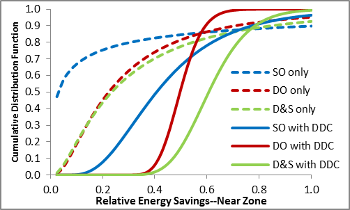
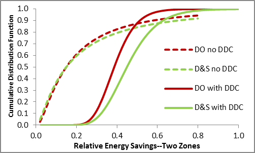
Chart 4 omits curves for Switching-Only (SO) controls, because there isn't enough daylight (even with IntelliBlinds™) to yield substantial savings over both zones.
IntelliBlinds™ dramatically increases the median relative savings with all types of lighting controls—by a factor of about 2 for DO controls, a factor of about 3 for D&S controls, and an order of magnitude for SO controls in the Near Zone.
Comparison with Relative Savings Observed in Independent Testing
Because few daylight-harvesting installations in the U.S. are equipped with DDC systems like the IntelliBlinds™ Model D, there is little independent real-world data on the savings potential of such systems. The best and most thoroughly documented source—although almost two decades old—remains the testing done at Lawrence Berkeley National Laboratory (LBNL).
In the 1990's, LBNL conducted several research programs to assess the energy and human factors implications of prototype dynamic daylighting systems—systems that combine Dynamic Daylight Control (DDC) with daylight harvesting capabilities. Despite being developed over a decade ago, the LBNL prototype systems still represent the state-of-the-art in conventional DDC technology, and the research remains among the most thorough and well-documented in the field.
LBNL's systems consisted of an interior-mounted adjustable shading device, a dimmable/switchable electronic ballast, various sensors, and a control computer. In some of LBNL's prototype systems, the adjustable shading device was an ElectroChromic (EC) smart window; in others, it was a motorized horizontal Venetian blind.
LBNL's research included long-term measurements in full-scale rooms as well as in a one-third-scale test cell representing a typical single-occupant office. The published results of the partial-scale testing are particularly useful because they include not just the relative savings, but also the absolute power and energy consumption figures for the baseline (no daylight harvesting), daylight-harvesting-only, and daylight-harvesting-with-DDC cases under near-identical conditions.
The partial-scale test data was collected on selected days from late May through mid-November in Berkeley, California, for both south and southwest window orientations, and using a variety of control protocols. The following chart summarizes the reported savings in lighting energy:
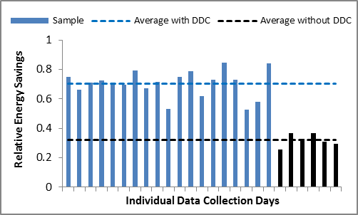
In the terminology used in the preceding discussion, the system tested by LBNL was a dual-zone D&S configuration, similar to the one assumed for the D&S CDF shown in Chart 4 above.
The 70% savings with DDC observed in LBNL's testing (Chart 5) are substantially greater than the 50% median savings of the modeled CDF (D&S "with DDC" curve of Chart 4), providing at least one independent data point that the with-DDC savings predicted by the relative savings model are acheivable in the real world. The greater savings observed in LBNL's testing could be due to any of several factors, including:
- Base-case slat tilt angle. LBNL's without-DDC data were collected with a slat tilt angle of about 70 degrees for most of the day (but then dynamically adjusted when the sun was within 5 degrees of the horizon), whereas the modeled CDF data assumes a fixed median slat tilt (based on independent research) of 40 degrees.
- Window orientation. The LBNL testing used south and south-west orientations, whereas the model assumes an average over all non-north orientations.
- Room geometry. In the partial-scale test room used in LBNL's testing, the sidelit zone was delimited by a wall located at 2.0 window-head-heights from the window, whereas the RDI data underlying the model was collected in a large space without a delimiting far wall. Our testing shows that the daylight reflected from a window-facing wall at the far edge of the sidelit area can significantly increase the savings.
- Median versus mean. While the median modeled savings of Chart 4 are 50%, the distribution is skewed so that the mean savings are closer to 60%.
Absolute Energy Savings
The absolute energy savings in kWh per square foot per year provided by daylight harvesting depend on the relative savings (per Charts 3 and 4), as well as the base-case lighting Energy Use Intensity (EUI), also expressed in kWh per square foot per year.
The EUI is the product of the installed Lighting Power Density (LPD) and the number of lighting hours per year. The number of lighting hours per year varies relatively little from office building to office building, but the LPD varies quite a bit depending on the vintage of the lighting system.
Lighting Energy Use Intensity (EUI) in New Construction and Major Renovation Scenarios
ASHRAE 90.1-2010, the current version of the energy efficiency standard for commercial buildings issued by the American Society of Heating, Refrigeration, and Air-Conditioning Engineers, specifies a maximum average LPD of 0.9 W/sf in office buildings. With 2,400 lighting hours per year—typical for domestic office buildings—this yields an EUI of 2.2 kWh/sf/yr. New construction and major renovations in major markets are typically required to comply with the latest standards, so our estimates assume an EUI of 2.2 kWh/sf/yr in those scenarios.
EUI in Retrofit Scenario
Because compliance with the latest standards is required only for new construction or major renovations, only a fraction of the existing building stock is compliant at any time, so the EUI in the retrofit scenario is significantly greater than in the new construction or major renovation scenarios. Here are three data points:
- As recently as 2003, the mean EUI in office buildings was as high as 6.8 kWh/sf/yr (EIA CBECS (2003),Table E6). Since many buildings have renovation intervals exceeding 10–15 years, it is plausible that many of the buildings surveyed in 2003 are still using the same lighting configuration.
- A 2010 study of the U.S. lighting market indicates an average EUI in office buildings of 4.1 kWh/sf/yr (Navigant 2012, Table 4.21).
- Based on a web search and an informal survey of office buildings in the Washington, DC metro area, the most frequently used luminaire configuration is a two-foot by four-foot (2x4) recessed parabolic troffer with three standard T-8 lamps and a first-generation electronic ballast, mounted on an 8-foot by 10-foot grid. This is also the same configuration generally assumed as the base-case in recent studies investigating lighting system upgrades. This configuration has an LPD of 1.1 W/sf—slightly lower than the 1.3 W/sf specified in 90.1-2001, and slightly higher than the current 0.9 W/sf standard. Assuming 2,400 lighting hours per year, this 1.1 W/sf LPD would result in an EUI of 2.6 kWh/sf/yr.
These three data points suggest a distribution of EUI in existing domestic office buildings that has a mean of 4.1 kWh/sf/yr and a mode of 2.6 kWh/sf/yr, as shown below:
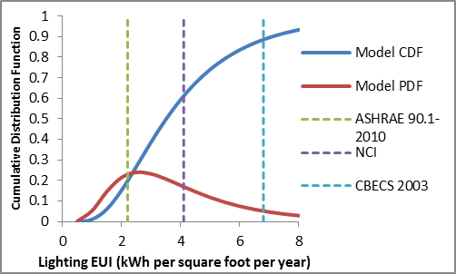
Per this distribution, 15% of the floor area in office buildings has an EUI greater than 6.0 kWh/sf/yr, more than twice as high as the mode of the distribution (2.6 kWh/sf/yr).
At the other extreme, the distribution also shows that 6% of the floor area has an EUI less than 1.5 kWh/sf/yr, or only about 70% of the 2.2 kWh/sf/yr implied by the current 0.9 W/sf LPD standard. This corresponds to an LPD of just 0.625 W/sf.
Investments in energy efficiency usually follow the path of quickest payback. Because the payback period of daylight harvesting with ordinary shading is longer than that of typical LPD-reducing lighting retrofits, an argument could be made that only buildings whose LPD is already relatively low would be candidates for daylight harvesting retrofits. According to this argument, only lower LPDs (e.g. the current 0.9 W/sf standard) should be assumed as a basis for estimating retrofit savings. However, our cost estimates are based on the EUI distribution over the entire stock of buildings, not just low-LPD ones, for three reasons:
- Adding IntelliBlinds™ significantly shortens the payback period for daylight harvesting, making it more appealing (either alone or as part of a comprehensive retrofit strategy) for higher-LPD buildings.
- LPD-reducing retrofits typically have a greater first cost than the simple daylight-harvesting configurations examined herein, which can offset some of the appeal of the shorter payback period.
- While LED technology is not yet cost-competitive with state-of-the-practice fluorescent technology in retrofit applications, the possibility that it will become cost-competitive within 5–10 years will deter some near-term investment in LPD reduction, increasing the relative appeal of other energy saving retrofits.
Cumulative Distribution Function (CDF) of Absolute Energy Savings
Combining the relative savings and lighting EUI distributions discussed above yields the following distribution of EUI savings from various daylight harvesting configurations across the potential sidelit space in U.S. office buildings:
These absolute EUI savings CDFs have the same shape as the relative savings CDFs of Charts 3 and 4. As with the relative savings, IntelliBlinds™ dramatically increases the absolute EUI savings with all types of lighting controls—by a factor of about 2 for DO controls, a factor of about 3 for D&S controls, and an order of magnitude for SO controls in the Near Zone.
Comparison with Distribution of Actual EUI Savings
Most of the published reports on the actual EUI savings from daylight harvesting each refer to the savings in a single daylit zone (or averaged over a single building). Because of varying assumptions and methodologies, it's difficult to infer a distribution of actual savings from these individual data points.
However, one 2005 study used the same assumptions and methodology to assess the actual savings in 123 sidelit zones (Sidelighting Photocontrols Field Study, 2005). This study is referred to herein as the SPFS. Of these 123 spaces, 59 were found to be generating positive savings, and all 59 of these "positive savings" data points are documented in the SPFS report. This is a sufficiently large sample to provide insight into the distribution of actual EUI savings from daylight harvesting.
The chart below shows the CDF of these 59 actual EUI savings data points, along with the previously shown CDFs of the projected savings for Switching Only (SO) controls (Chart 7) and Dimming-Only (DO) controls Chart 8:
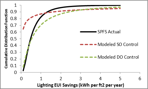
The SPFS and projected CDFs differ significantly for four reasons:
- The 59 daylit spaces of the SPFS included a mix of SO and DO lighting controls, while the projected CDFs are for a single type of daylighting control. However, the same methodology can be used to develop a projected CDF for the same mix of controls used in the SPFS.
- The CDF derived from the SPFS data doesn't reflect the entire population of 123 assessed daylit spaces, but rather only the spaces that were providing positive savings. In contrast, the projected savings CDFs reflect the entire popluation, including the proportion with negligible savings. This can be accounted for by shifting the projected CDFs right so that the minimum savings exceed some small non-zero value (5% was assumed in this analysis).
- The 59 daylit spaces of the SPFS included a mix of shaded and unshaded windows (the latter of which were mostly north-facing), while the projected CDFs assume only shaded windows with sunny exposures. Despite being mostly north-facing, the unshaded windows of the SPFS yielded 16% greater savings than the shaded sunny windows. This 16% margin can be added to the median of the projected savings CDF to reflect the same mix of shaded and unshaded windows.
- The 59 daylit spaces of the SPFS had a mean installed Lighting Power Density (LPD) of 1.0 Watt, while the mean LPD assumed in the projections is 1.7 Watt (based on the mean EUI of 4.1 kWh from Chart 6, divided by an assumed 2,400 lighting hours per year). Dividing the median of the projected CDF by 1.7 can account for this difference.
The following chart shows the impact of adjusting the projected CDF savings to account for these four factors:
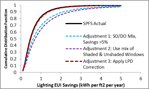
Obviously, the close agreement between the actual and adjusted projected CDFs doesn't fully validate the projected EUI savings, but shows that they are at least consistent with real-world data as reported in the SPFS.
Dollar Savings
In addition to the reduction in lighting EUI (kWh per square foot per year), the dollar savings from daylight harvesting also depend on the local electricity rate schedule. And if the rate schedule includes demand or Time-Of-Use (TOU) pricing, the dollar savings also depend on the reduction in lighting power (W per square foot) and when it occurs.
Average Electricity Price
The U.S. Energy Information Administration (EIA) tracks the average retail price of electricity by sector, state, and utility provider. The average retail price is defined as the total revenue (including both consumption and demand charges) divided by the total sales in kWh.
Unfortunately, the EIA doesn't provide explicit data on the distribution of the average retail price across commercial buildings. However, the EIA also administers the Commercial Buildings Energy Consumption Survey (CBECS), and the data reported therein can be used with the retail price data to infer a price distribution. Such an analysis yields the following approximate CDF of average retail electricity price across commercial buildings in the USA:
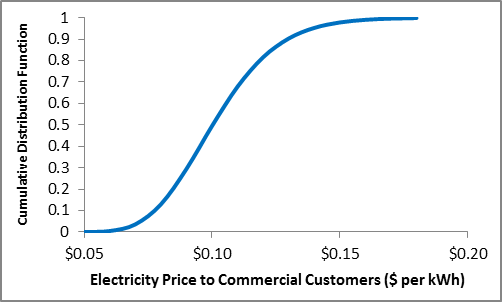
The median price is $0.100 per kWh, while the mean price is about $0.102 per kWh.
Impact of Demand and Time-Of-Use (TOU) Pricing
While the EIA's average retail price in $ per kWh includes both consumption and demand charges, it doesn't necessarily represent the dollar savings that would occur from a unit reduction in consumed kWh.
For example, if a kWh reduction occurs by reducing the "on" time of equipment that runs during off-peak hours, then there will be no savings in demand charges (if demand pricing is in effect), or the dollar value of the kWh savings will be based on a relatively low off-peak rate (if TOU pricing is in effect). In this scenario, multiplying the kWh reduction by EIA's average retail price will over-estimate the actual dollar savings.
On the other hand, if a kWh reduction occurs by reducing the kW load when local electricity demand is highest, then demand charges will be reduced (if demand pricing is in effect), or the dollar value of the kWh savings will be based on a relatively high peak rate (if TOU pricing is in effect). In this scenario, multiplying the kWh reduction by the EIA's average retail price will under-estimate the actual dollar savings.
The latter scenario applies to daylight harvesting: in most regions of the USA, peak electrical demand and peak TOU rates occur in summer afternoons, which is exactly when daylight harvesting yields the greatest reduction in lighting power (kW). So, multiplying the EUI savings by the EIA's average retail price will under-estimate the actual dollar savings for daylight harvesting. This under-estimation can be approximately corrected by multiplying the EIA's average retail price by a factor equal to F*(1-R) + R, where
- F is the median fraction of hours per year which incur demand charges
- R is median ratio of total electricity charges to consumption-only charges
Fraction D of Hours per Year Incurring Demand Charges
As previously noted, the EIA's average retail electricity price includes demand as well as consumption charges. So, if the annual demand charges in the EIA's database were accrued evenly over each of the 8,760 hours per year, then multiplying the EIA's average retail price by the annual savings in EUI would yield a reasonably accurate estimate of the total annual dollar savings from daylight harvesting.
However, demand charges are incurred over only a small fraction of the hours in a year. The smaller the fraction of time over which the demand charges were accrued in the EIA's database, the greater the actual dollar savings for daylight harvesting relative to the product of the EIA price and the annual EUI savings.
Over most of the continental USA, peak electrical demand in commercial buildings occurs during summer afternoons. So, for most buildings, the bulk of the annual demand charges are due to about one-quarter of the hours of about one-quarter of the days in the year, or about 6 percent of the hours per year. Thus, D is about 0.06.
Ratio of Total Electricity Charges to Consumption-Only Charges
Demand charges represent a significant fraction of the total electricity costs in commercial buildings. For example, one published source (Arnold, 2003) reports the ratio of demand charges to overall electricity charges for a typical office building served by eleven investor-owned utilities. The complement of this ratio is the ratio of consumption charges to total electricity charges. The reciprocal of that complement, in turn, is the ratio R of total electricity charges to consumption charges, and has the following Cumulative Distribution Function (CDF):
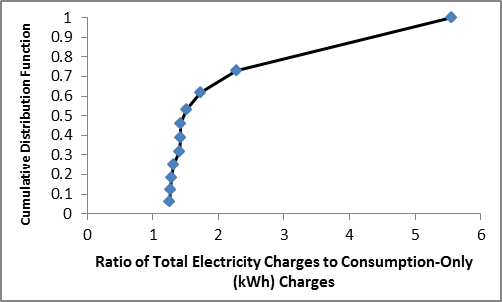
The median and average values of R are 1.43 and 1.86, respectively, meaning that a typical total electricity bill in the sample population is 43% greater than the consumption charges alone. This suggests that, for an energy saving measure that reduces both kWh and peak kW by roughly the same proportion (such as daylight harvesting), the median and average total dollar savings will be about 43% and 86% more, respectively, than the savings in consumption charges alone.
Marginal Dollar Value per kWh Savings from Daylight Harvesting
The methodology and values of D and R discussed above indicate that the marginal dollar value of a unit kWh savings from daylight harvesting—assuming a proportionate reduction in peak kW—is about 1.4 times the EIA's average retail price per kWh to commercial customers.
Distribution of Dollar Savings Across Potential Sidelit Area
Combining the EUI savings and EIA average price distributions with the Demand/TOU pricing factor discussed above yields the following distribution of dollar savings from various daylight harvesting configurations across the potential sidelit space in U.S. office buildings:
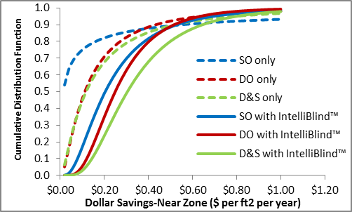
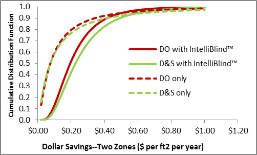
Of course, these absolute dollar savings CDFs have the same shape as the relative savings CDFs of Charts 3 and 4 and the EUI savings CDFs of Charts 7 and 8. As with the relative and EUI savings, IntelliBlinds™ dramatically increases the dollar savings with all types of lighting controls—by a factor of about 2 for DO controls, a factor of about 3 for D&S controls, and an order of magnitude for SO controls in the Near Zone.
Costs
As with the savings, the costs of an energy saving product depend on many installation-specific variables, leading to a distribution of costs over the potential installed base. For the daylight-harvesting configurations considered herein, the effective cost per unit floor area depends primarily on five factors:
- The per-system costs of the required equipment
- The purchasing scenario (e.g. retrofit versus new construction)
- The value of applicable rebates or tax incentives
- The floor area covered by the daylight-harvesting lighting control
- The floor area covered by each IntelliBlinds™ unit.
The latter factor dominates the variance in the total system costs. Therefore, it's treated as a distribution, while median values are used for the other four factors.
The subsequent paragraphs discuss the basis for estimating each factor and provide a summary of the resulting cost distributions.
Per-System Costs: Daylight Harvesting
The costs of daylight harvesting equipment vary over a wide range depending on the type and complexity of the installation. For the stand-alone single-zone and dual-zone systems considered here, however, the cost variance is small. The median prices assumed herein are for specific makes and models of lighting control, and were estimated by applying a typical quantity discount factor to the single-quantity prices obtained via a web search.
Per-System Costs: IntelliBlinds™
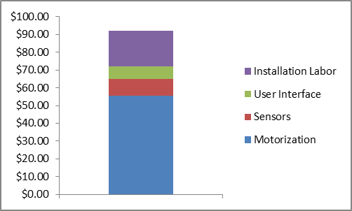
IntelliBlinds™ costs are based on the Bill of Materials for the reference Model D design, assuming volume production and a 200% mark-up from production to end-user cost (i.e. the end-user cost assumed in the cost and payback estimates is 300% of the production cost). The following chart provides a summary breakdown of the retail price per unit (including mark-up):
Purchasing Scenario
The effective cost of an energy saving product depends on why it's being purchased:
- If it's being bought primarily to replace an installed device that's worn-out or obsolete—or for new construction or a major renovation—then the effective price is just the incremental installed price beyond a less efficient alternative product. This is the replacement/new construction scenario.
- On the other hand, if it's being bought primarily for energy savings—and if there's already a less-efficient installed device with signficant remaining life—then the effective price is the total installed price of the new product, plus the depreciated value of the existing product. This is the retrofit scenario.
Obviously, costs are greater in the retrofit scenario. But every building is a candidate for a retrofit, whereas only a small percentage of the commercial floor area is fully renovated or newly constructed each year. So retrofit cost-effectiveness is the holy grail for every energy saving building technology. The IntelliBlinds™ Model D was developed specifically for retrofit applications, and the costs discussed here are exclusively for the retrofit scenario.
Incentives
Incentive programs to stimulate energy efficiency have proliferated to the extent that most daylight harvesting projects now qualify for some sort of rebate, tax deduction, or tax credit. However, because tax deductions and credits for energy efficiency have been changing frequently, the incentives considered herein are limited to utility sponsored rebate programs (which appear relatively stable).
Rebate programs are either prescriptive (in which a fixed benefit is provided for each prescribed energy saving technology or measure), or savings-based (in which the benefit is based on the actual kW or kWh reduction). Most prescriptive programs explicitly list daylight-harvesting equipment among the qualifying technologies, but only a few list automated shading systems. However, most prescriptive programs also offer a "custom" provision that can provide benefits for any demonstrably effective energy saving technology, including automated shading. And some prescriptive programs provide benefits based on LEED points, which can be earned by automated shading devices as well as daylight-harvesting lighting controls.
Based on an informal web survey, the following rebates are assumed herein, and are intended to represent the median dollar value of applicable rebates available in the USA:
- Lighting control photosensor: prescriptive rebate, $20 per unit
- Dimming ballast: presescriptive rebate, $40 per unit
- Automated shading: custom rebate, $0.10 per kWh savings
Floor Area per Daylight Harvesting Lighting Control
The stand-alone single-zone and dual-zone daylight harvesting lighting controls considered here require one photosensor/controller per system and one dimmable ballast/switch per zone, with each zone controlling a single luminaire. The greater the illuminated area per controlled luminaire, the lower the cost per unit floor area of the daylight-harvesting lighting control.
Based on a web search and an informal survey of buildings in the Washington, DC metro area, the most frequently used luminaire configuration in existing office buildings is a two-foot by four-foot (2x4) recessed parabolic troffer with three standard T-8 lamps and a first-generation electronic ballast (for a total luminaire power requirement of 88 W), mounted on an 8-foot by 10-foot grid. This is also the same configuration generally assumed as the base-case in recent studies investigating lighting system upgrades. This 88-W 80-sf configuration has an installed Lighting Power Density (LPD) of 1.1 W/sf, which is equal to the mode of the LPD distribution assumed in our savings estimates.
Other linear-fluorescent luminaire configurations include two and four-lamp 2x4's, two-lamp 2x2's, and single-lamp recessed and suspended fixtures; other luminaire spacings include 8x8, 10x10, and 10x12 feet. However, the 8x10 spacing appears dominant in existing office buildings, and appears close to the median and mean of what seems to be a roughly normal distribution of areas-per-luminaire in existing buildings.
Therefore, our cost estimate is based on median illuminated area of 80 square feet per luminaire, yielding an assumed floor area of 80 square feet for a single-zone system and 160 square feet for a two-zone system.
Because the LPD and the illuminated area per luminaire are not statistically independent quantities, and because our savings estimates treat the LPD as a distribution, our cost estimate is based on only the median area-per-luminaire (with zero variance) to avoid exaggerating the variance in the resulting payback-period distributions.
Floor Area per IntelliBlinds™ Unit
The floor area that can be sidelit per IntelliBlinds™ unit depends on two variables:
- The height of the head (i.e. top) of the host window determines the depth of the sidelit area per IntelliBlinds™.
- The width of the host blind determines the width of the sidelit area per IntelliBlinds™.
Sidelit Area Depth
Our cost estimates assume a ratio of 1.0 of sidelit depth to window head height for single-zone systems, and a ratio of 2.0 for dual-zone systems. These are the same depth-to-height ratios used in IntelliBlinds™ testing and are also consistent with the codes and standards that address daylight harvesting (e.g. IECC-2009, ASHRAE 90.1, and California Title 24). The ratios are arguably conservative for a sidelighting installation that includes Dynamic Daylight Control (DDC), because DDC tends to increase the uniformity of daylight in a sidelit space.
The other factor in the sidelit area depth—the window head height—varies from building to building. Unfortunately, window head height statistics are not among the wide range of commercial building characteristics tracked by the EIA's periodic Commercial Buildings Energy Consumption Survey (CBECS). However, a published study of 59 sidelit spaces on the west coast does provide information on the distribution of window head heights across a reasonably large sample population (Sidelighting Photocontrols Field Study, 2005, Figure 48, page 95). Analyzing that data yields the following Cumulative Distribution Function of window head heights in sidelit spaces:
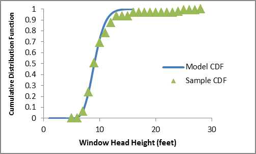
Multiplying the window head heights of Chart 16 by assumed factors of 1.0 and 2.0 yields the distributions of sidelighting depths for single-zone and dual-zone systems, respectively, assumed in our cost projections.
Sidelit Area Width
The aforementioned commercial building standards that address sidelighting define the width of the sidelit zone as the window width plus a constant 2 feet on either side of the window (for a total of the window width plus 4 feet), subject to the absence of vertical obstructions in the sidelit space.
However, the area that can be sidelit by each IntelliBlinds™ unit is limited by the width of the host miniblind, rather than by the width of the window. This is because extremely wide windows, e.g. strip windows, can require more than one miniblind, and hence more than one IntelliBlinds™.
So, the sidelit area per IntelliBlinds™ unit is based on miniblind width vice window width. And rather than apply an addend of 4 feet to the miniblind width, our cost estimates apply a factor of 1.5 to obtain the sidelit area width. The use of a factor vice an addend facilitates estimation of the distribution of the net effective costs and paybacks.
For miniblinds with widths smaller than 8 feet, this factor of 1.5 yields a smaller sidelit width than the width-plus-4-feet specified in the standards (and thus over-states the IntelliBlinds™ cost per square foot), while for windows wider than 8 feet, the factor of 1.5 yields a larger sidelit width than the standard (and thus under-states the cost per square foot).
Unfortunately, while there are statistics on the window-to-wall ratios in existing buildings, information on the distribution of installed miniblind widths is not readily available in the public domain. Short of administering a large-scale survey, the only practical way to obtain statistically ample information on the distribution of blind widths appears to be via photogrammetric analysis of building facades. Such an analysis, performed on the results of an internet image search on "office building", suggests the following distribution of miniblind widths:
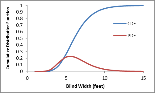
The median and mean widths are 6 feet and 6.2 feet, respectively. Note that, because both of these central tendency metrics are less than 8 feet, our assumed factor of 1.5 for the miniblind-to-sidelit width is more conservative (i.e. yields a smaller sidelit area, and thus a greater IntelliBlinds™ cost per square foot) than the width-plus-foor-feet specified in the applicable standards.
Summary of Estimated Costs
The following tables summarize the estimated median daylight-harvesting costs in a retrofit scenario:
| Daylight Harvesting Only | Daylight Harvesting plus IntelliBlinds™ | Daylight Harvesting plus Conventional DDC | ||||||
|---|---|---|---|---|---|---|---|---|
| Switching Only | Dimming Only | Dimming and Switching | Switching Only | Dimming Only | Dimming and Switching | |||
| No Rebates | Single Zone | $0.78 |
$1.48 | $1.73 | $1.88 | $2.55 | $2.79 | $5.05 |
| Dual Zone | $0.43 |
$1.11 | $1.24 | $0.97 | $1.64 | $1.76 | $2.87 | |
| Typical Utilty Rebates | Single Zone | $0.53 | $0.73 | $0.98 | $1.49 | $1.72 | $1.93 | $4.31 |
| Dual Zone | $0.31 | $0.49 | $0.62 | $0.82 | $0.94 | $1.04 | $2.24 | |
| Note 1: Unlike the lighting control costs, the estimated DDC costs have a significant variance due to the relatively broad distribution of miniblind widths and window-head-heights in existing buildings, which in turn leads to a relatively broad distribution of sidelit area per system. This variance is not listed in this table, but is reflected in the payback period distributions presented herein. | ||||||||
Payback Periods
The dollar savings and cost distributions discussed above can be used to estimate the distribution of simple payback periods for daylight harvesting retrofits across the entire aggregate office building floor area in the U.S. As with many other energy saving technologies, the resulting payback distributions span a huge range, extending from months to decades.
However, given the market's current sensitivity to payback period, daylight harvesting retrofits—with or without IntelliBlinds™—don't make sense in buildings with very low Lighting Power Densities (LPDs) or utility rates. And IntelliBlinds™ isn't as cost effective when used on small blinds. So excluding such installations yields a more realistic distribution of actual paybacks.
For example, a prime candidate building for an IntelliBlinds™ retrofit might have the following characteristics:
- An LPD of at least 1.46 Watts per square foot. This is the median LPD in existing office buildings, and is significantly lower than the mean (1.7 Watts). It's likely that daylight harvesting would be used in many buildings with higher LPDs, too, but there is increasing likelihood of competition with major LPD-reducing retrofits as the LPD increases.
- Electricity consumption charges of at least $0.12 per kWh, with a ratio of total charges to consumption charges of 1.9. This consumption charge is at about the 80th percentile for U.S. office buildings, but is very typical of the commercial rates in major metropolitan areas. The ratio of total to consumption charges appears to be the average for commercial electricity rate structures in the U.S.
- A miniblind width of at least 7 feet and window head height of at least 9 feet. This width is at about the 80th percentile for U.S. office buildings, while the window head height is roughly the median value.
The following charts show the quartiles of the projected paybacks for such retrofits in single-zone and dual-zone configurations:
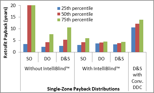
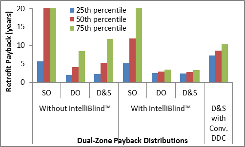
The quartile charts are informative because the median (50th percentile) paybacks correspond to the inverse of the expected ROIs, while the payback distributions (i.e. the spread between the 25th, 50th, and 75th percentile paybacks) reflect the risks associated with achieving those ROIs.
As shown in in Charts 18 and 19, even in "prime" installations, the payback distributions for daylight harvesting alone (without DDC) are broad—especially for Switching-Only (SO) lighting controls. Adding DDC tightens the distributions considerably by eliminating the over-shading losses. However, conventional DDC technology is so expensive that it lengthens the median paybacks. The IntelliBlinds™ Model D, on the other hand, is inexpensive enough to shorten the median paybacks while it tightens the distributions. The impact is particularly significant for SO controls in single-zone configurations and for both DO and D&S controls in dual-zone configurations, where IntelliBlinds™ can turn what would otherwise be an unattractive or marginally attractive investment into a highly attractive one.
Summary of Key Points
- The IntelliBlinds™ Model D saves energy primarily by increasing the average level of useful daylight that can be harvested (thereby reducing lighting energy consumption), and secondarily by reducing thermal loads (thereby reducing HVAC energy consumption)
- As with any other energy saving device, the actual savings will depend on numerous installation-specific variables. However, projecting the savings is straightfoward and can be done mostly with publicly available data
- The resulting savings projections are consistent with published savings data for other DDC systems, as well as with the savings shortfalls observed in daylight harvesting systems without DDC
- The projections show that IntelliBlinds™ will more than double the kWh and dollar savings from daylight harvesting, while significantly reducing the distribution and median of the payback periods. The result will be a dramatic improvement in the economics of daylight harvesting in typical installations